
Use Excel’s FILTER function when you need a second, live view of selected rows while keeping the full source list visible. Unlike the Filter button on the Data tab, which hides non-matching rows in the original range, FILTER returns matching rows in a new location.
This is useful for a task tracker that needs a separate list for one owner, a report that shows only open items, or a simple dashboard area. Change the criteria cell and the returned list updates automatically; the original table is untouched.
FILTER versus the Data tab Filter button
| Need | Better option |
|---|---|
| Temporarily focus on rows in the source table | Data tab Filter (AutoFilter) |
| Keep the source visible and show a separate subset elsewhere | FILTER function |
| Let a report area change when a criteria cell changes | FILTER function |
| Manually narrow a table using column drop-downs | Data tab Filter (AutoFilter) |
AutoFilter can be applied to a range or table and hides rows that do not meet its criteria. FILTER is a worksheet formula that produces a new dynamic-array result instead. Microsoft documents the distinction through its separate guidance for filtering data in a range or table and its FILTER function reference.
Set up the source and output area
FILTER is available in Excel for Microsoft 365, Excel 2021, and Excel 2024. For a recurring worksheet, format the source records as an Excel Table with a clear name such as Tasks. Tables make structured references easier to read and expand as records are added.
Put the FILTER formula in an ordinary blank cell outside that table. A dynamic-array formula can use a table as its source, but spilled array formulas are not supported inside a table. Leave sufficient empty cells beneath and to the right of the formula for the results.
The formula shape
=FILTER(array, include, [if_empty])- array is the range or table columns to return.
- include is a row-by-row TRUE/FALSE test. Rows whose test is TRUE are returned.
- [if_empty] is optional text or another value to return when no rows match.
The square brackets mean the third argument is optional, not that you type brackets into the formula. Supplying a clear no-results message is usually friendlier than leaving the empty case unhandled.
Build a one-condition live list
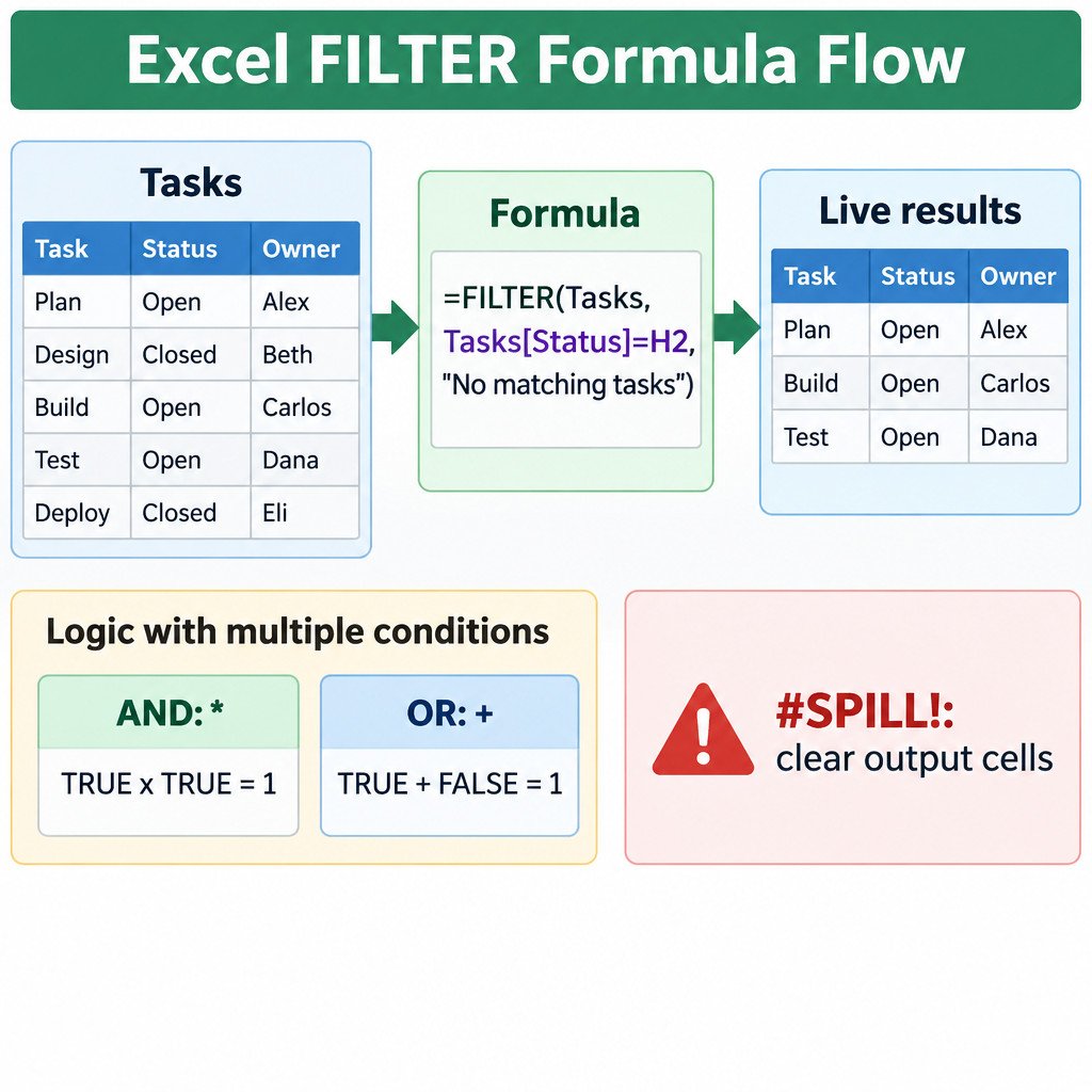
In this illustrative task-tracker example, Tasks is an Excel Table with columns including Status. Cell H2 contains the status to display, such as Open.
=FILTER(Tasks,Tasks[Status]=H2,"No matching tasks")Tasks tells Excel to return all columns in every qualifying row. Tasks[Status]=H2 tests each value in the Status column against H2. The result begins in the formula cell and spills into the cells needed for all matching rows and columns.
Require two conditions with AND
Suppose H2 contains an owner and H3 contains a status. To return tasks that belong to that owner and have that status, multiply the two tests:
=FILTER(Tasks,(Tasks[Owner]=H2)*(Tasks[Status]=H3),"No matching tasks")In Excel’s logical array calculation, TRUE behaves as 1 and FALSE as 0. Multiplication returns 1 only when both tests are TRUE: 1 × 1 = 1. Any combination containing FALSE becomes 0, so that row is excluded.
Accept either condition with OR
Use addition when either test should qualify a row. This illustrative formula returns a task if its Owner equals H2 or its Status equals H3:
=FILTER(Tasks,(Tasks[Owner]=H2)+(Tasks[Status]=H3),"No matching tasks")A row that meets one or both tests has a non-zero result and is included. Be deliberate here: OR can produce a much broader list than AND. It is appropriate for a queue such as “items assigned to me or items marked urgent,” not for a request that both conditions must be true.
Sort the separate result without changing the source
FILTER preserves the source order. If the report list should be sorted independently, wrap it in SORT:
=SORT(FILTER(Tasks,Tasks[Status]=H2,"No matching tasks"))This sorts the returned output, not the underlying Tasks table. For a custom sort column or descending order, use SORT’s additional arguments after confirming which output column you intend to sort by.
Microsoft’s FILTER function documentation confirms the syntax, Boolean include logic, AND/OR operators, and the option to combine FILTER with SORT.
Fix the errors that stop a live list
#CALC! when nothing matches
If FILTER finds no matching rows and you omitted [if_empty], Excel can return #CALC!. Add a third argument such as "No matching tasks". This makes an empty result understandable without masking other formula problems.
#SPILL! because the output area is blocked
A spilled result needs empty cells. Clear values or formulas in its expected output area, unmerge any cells that intersect it, and move the formula if the result would run beyond the worksheet edge. Do not place the formula inside an Excel Table. Excel’s error indicator can identify obstructing cells in many cases.
Errors caused by the include test
The include test must line up with the filtered array: when filtering rows, it needs one result for each source row. Also check the source columns for errors such as #N/A or #VALUE!; an error in the include array can propagate into FILTER rather than simply excluding that row.
Before you share the workbook
- Test a matching criterion, a no-match criterion, and a criterion with several matches.
- Leave the entire potential spill range clear; the list may grow when source records are added.
- Check that the criteria cells use the same values and spelling as the source data.
- Keep the formula outside the source table, while using the table for structured references where useful.
- Confirm recipients use an Excel version that supports FILTER.
- If the formula refers to a dynamic array in another workbook, keep the source workbook open when refreshing the linked result.
FILTER is best thought of as a live report formula: it creates a new view, while AutoFilter changes the view of the source itself. Once the source, criteria cells, and spill area are set up cleanly, the same pattern can power many small reporting tasks without copying rows by hand.
